Table of Contents
Class Prep
Class 1
Class 2
Class 3
Class 4
Class 5
Class 6
Class 7
Class 8
Class 9
Class 10
>>Topical Articles<<
Assumed Longitude
Bowditch
Bygrave
Casio fx-260 Solar II
Emergency Navigation
Making a Kamal
Noon Sight
Pub. 249 Vol. 1
Sextant Adjustment
Sextant Skills
Sight Averaging
Sight Planning,
Error Ellipses,
& Cocked Hats
Slide Rules
Standard Terminology
Star Chart
The Raft Book
Time
Worksheet Logic
BCOSA.ca
The geographic points (GPs) of celestial objects move across the face of the earth at the rate of 360° per 24 hours, or 15° per hour...which works out to 1° every
four minutes. While the slope a celestial object follows (i.e. its angle to the horizon) varies continuously throughout the day, over any given 4 minutes period it can be treated — to the
degree of accuracy delivered by sextant navigation — as a straight line.
The overall process of sight averaging is to:
After inputting our DR position, with the data from the Nautical Almanac, we come up with a meridian angle of 52° 36.5'.
Once we do our sight reduction calculations, we come up with an Hc for the first sight of 37° 17.1'.
We rerun our sight reduction calculations, but this time using a meridian angle of 51° 36.5', which represents the passage of 4 minutes of time.
We come up with an Hc for this second sight of 38° 16.3'.
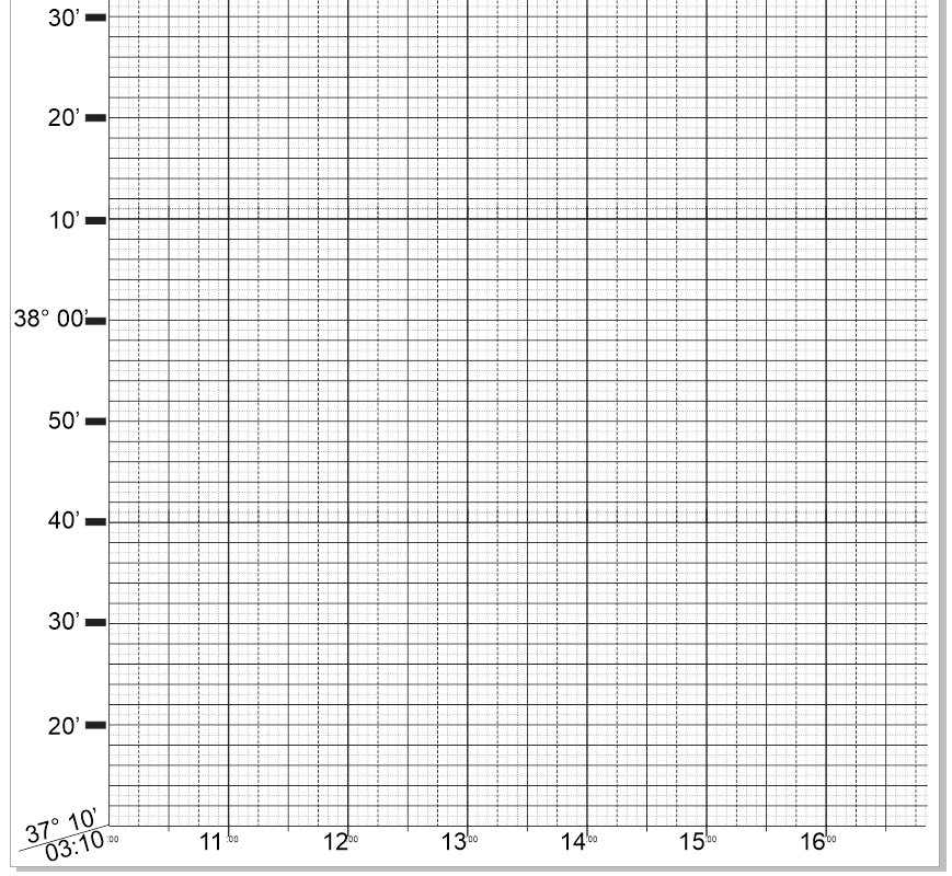
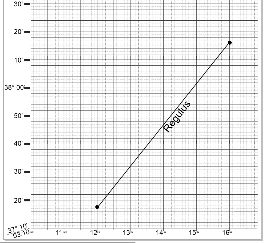
Now we need to plot all the data. We start by setting up the plotting sheet so it covers the time period we are interested in, and the range of heights you have. Next, we plot our two Hc values, which gives us the slope of Regulus over a 4 minute period which overlaps the period when we collected our four observations.
So as to avoid overlapping this line with our actual data, we can lay out this line using the times of 3:12 to 3:16. Which minutes we use is not critical. We are
interested in the slope of the line...the ratio of time to altitude gain of the star Regulus.
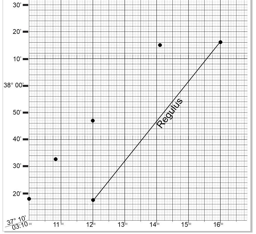
Plot the four data points of the sights we took. We use the raw Hs values. We don't worry about dip or any other corrections. As long as we treat all four sights
the same way, we can compare their slope to our calculated slope for Regulus.
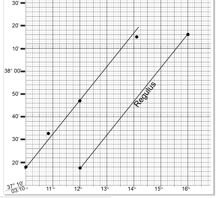
Use your parallel rule to transfer the calculated slope over to your sight data, and aim for a best-fit.
What we observe from this data is that the first and third sights are likely to be pretty accurate.
The second shot we took was a little high, and the fourth shot was several minutes too low.
Since we have already done our Nautical Almanac work for 03:10:00, we will choose to use the first
shot rather than the third.
It sometimes happens that after we get our best-fit for the slope, there are no sights that lie
precisely along the line. We might have something that looks like this:
What we can do in this case is to pick a hypothetical sight that lies precisely on the line. I have
used this "hypothetical shot" technique in the past and ended up with a fix that agreed precisely
with my GPS.
If you use a hypothetical shot, just fill in that value for Hs on your worksheet, and continue
with all your other calculations, and plotting of LOPs, as normal.
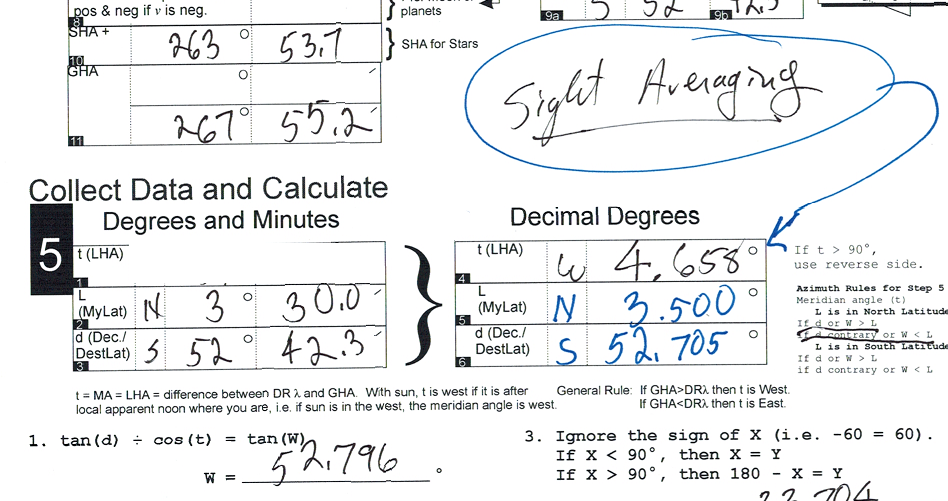
You can use this technique for sight averaging whether you are using Pub. 249 for your sight reduction, or using
the Bygrave equations. If either case, if the object is west of you, the meridian angle is increasing at the rate
of 1° per 4 minutes. If it is east of you in the sky, the meridian angle is decreasing at that rate.
So if you are using equations to do your sight reduction, you will start by running the equations for the first shot in your
sequence of four sextant sights.
So for example, here are four sights of the star Regulus taken with an artificial horizon on November 22, 2019 starting at 03:10, from 3° 30.0' N, 113° 51.0' W.


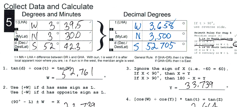
In this case, you can see that "t" is "West", so the value of t is increasing. To sort out the altitude of this object after the passage of 4 minutes of time, simply add 1° to the value of "t" and recalculate.
If you are using Pub. 249, this particular process takes less time than if you are using Bygrave equations. Once you have done the work to come up with an Hc value for a given LHA (or "t")...
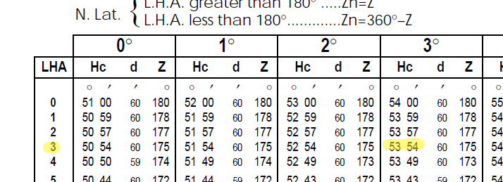
...then you can get a value for four minutes of time later by simply picking and LHA/t that is 1° different:

(For purposes of sight averaging, you don't need to worry about the d or Z values in Pub. 249. All you need is the change in Hc.)